Future of the Oxford Cambridge Arc

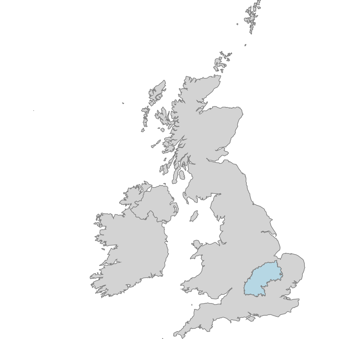
What is the Oxford Cambridge Arc?

The Oxford Cambridge Arc in a region in south central England that runs between Oxford and Cambridge via Milton Keynes and four major settlements including Cambridgeshire, Bedfordshire, Buckinghamshire and Oxfordshire. It is home to 3.7 million people, generating over 2 million jobs and contributing over £110 billion of annual Gross Value Added (GVA) to the UK economy per year. The area also contains some of the fastest growing and most productive towns and cities in the UK.

Future Development Scenarios

A report published in 2018 by the National Infrastructure Commission outlined substantial plans to increase access and connectivity to the Arc area by 2050. This vision includes one million new homes across the Arc, an east-west Expressway road, and major improvements to rail routes. However, in order to learn more about how this vision would actually impact urban development, the Infrastructure Transitions Research Consortium (ITRC) team simulated possible futures of the Arc through computer modelling. This article will outline the steps of the analysis in more detail. To get started, the team first defined four high-level future scenarios based on the vision by making assumptions about the number of new homes and transport that will need to be build, where they will be built, and constraints on how much development can take place. The four scenarios are compared to a baseline representing the preesent day.

Overview of Scenarios

1. Existing Expansion (Grey Policy)
2. Existing Expansion (Green Policy)
3. New Settlements (Grey Policy)
4. New Settlements (Green Policy)

Select a scenario to learn more.

Select Scenario

The baseline assumes that population will be based on recent growth rates and housing on recent average dwelling completion rates. There will be no intra-city transport system built.

The expansion grey scenario assumes that existing cities will expand due to inward migration and good intra-city transport systems will be built. The grey policy puts less constraints on development in favour of higher density.

The expansion grey scenario assumes that existing cities will expand due to inward migration and good intra-city transport systems will be built. The green policy puts more constraints on development to preserve natural capital.

The new settlements scenario assumes that new cities will emerge with major growth in five new urban conurbations (clusters of smaller cities) and good intra-city transport systems will be built. The grey policy puts less constraints on development in favour of higher density.

The new settlements scenario assumes that new cities will emerge with major growth in five new urban conurbations (clusters of smaller cities) and good intra-city transport systems will be built. The green policy puts more constraints on development to preserve natural capital.

The Urban Modelling Process

Using the future scenarios as a starting point, we can start to test out the theories and assumptions made through computer-based simulations. While we can’t fully capture every nuance about the future built environment, analyzing and visualising the trade-offs can help planners and policy-makers make informed decisions. One of the modals used to assess the Arc is called the Urban Development Model (UDM). We will take a brief moment to explain the general process of the UDM before showing the results applied to the Arc.

Overview of UDM Process Steps

1. Identify elements of the environment
2. Calculate current dwelling densities
3. Calculate ecosystem services
4. Identify constraints
5. Introduce future built environment features
6. Calculate attractiveness scores
7. Identify development suitability
8. Identify future dwelling density
9. Allocate future development
10. Calculate land use metrics

Scroll through each step to learn more about the UDM.

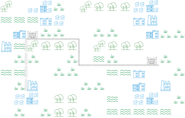
Step 1. Identify elements of the environment

←

→

Define existing urban land features (e.g. residential buildings) and non-urban land features (e.g. green space).

Calculate the urban land features based on density per grid cell. Areas with more dwellings will have a higher density.

Calculate the value of non-urban land features based on the ecosystem services needed to help maintain it. A verge by a road has value for flood protection, air quality, and recreation.

Define areas where development should be restricted, such as historical sites or the protection of nature and wildlife.

Layer on plans for new development where there is a location in place to test assumptions (i.e., new rail stations, road nodes, settlement centres). Exclude individual homes because we do not yet know where they will be distributed.

Identify the areas best suitable for living by defining factors that will attract people to move to the Arc (i.e. proximity to employment or green space) and assigning each a ‘weight’.

Combine the attractors and constraints to assess whether a an area of land is suitable for development, and which to prioritize. This measure of suitability considers the weight of each attractor in step 6, and blocks off cells with constraints in step 4.

Figure out how much development can actually take place by assigning options based on how many people can “fit” into undeveloped land based on proximity to urban centers or public transport. This often results in hotspots around town centers and business districts with high density.

Apply the urban development model to allocate future development at the identified densities (the most suitable areas first) to get a prediction of where development will actually take place.

Summarize results in a way that helps government authorities and planners make decisions by replacing the cell grids with administrative boundaries that map to different policy areas.

Applying Urban Modelling to the Arc Scenarios

Now that we have an understanding of the urban modelling process, let’s look at how it was applied to the Arc. We will go through the process one step at a time. For each step we will compare results at three different scales (Arc, city, neighbourhood) in order to compare both the bigger picture and details.

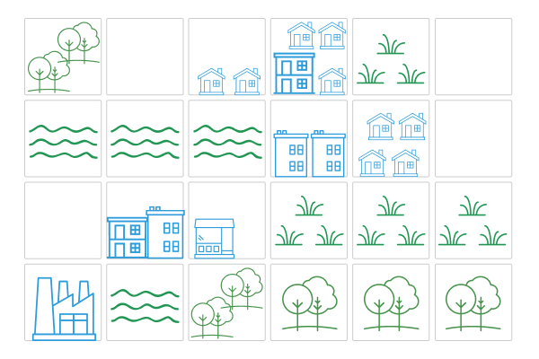
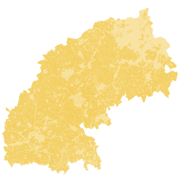
Step 1: Identify elements of the environment

Existing urban land features (in blue) and non-urban land features (in green).

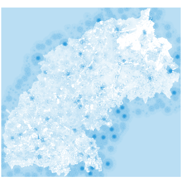
Step 2: Calculate current dwelling densities

Areas with more dwellings will have a higher density. This is represented by the blue cells, where the darker blue represents a higher density; the lighter blue the lower density.

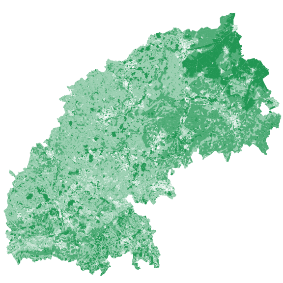
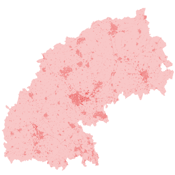
Step 3: Ecosystem services in the Arc

Change Scale

Insert legend image

Aspects of natural capital in the Arc include parks, grasslands, woodlands, verges, and any other aspect of green space, land uses, and habitats. The darker green represents higher quality ecosystem services.

Step 4: Identify constraints

Insert legend image

We introduce constraints to protect nature, wildlife, historical landmarks, and areas which are not feasible to develop. We “block off” these areas from development.

Step 5: Identifying future built environment features

Improvements to the transport links between Oxford and Cambridge are a key aspect of the future vision for the Arc. Future plans include a new expressway and East West Rail (EWR) will link Oxford and Cambridge. While the baseline scenario would not see any changes, the other scenarios would have rail stations and road nodes. New settlements would also include new settlement centres.

Step 6. Calculate attractiveness scores

Insert legend image

Attractors are things that will drive more people in to the Arc. Such attractors could include information on the performance of local schools, local accessibility (distance) to shops, services or transport hubs.

Step 7. Suitability of land for development

Insert legend image

Based on the weighing of both the attractors and contraints, the output of the UDM is a combined set of development suitability scores based on selected spatial scenarios and the combination of attractors and constraints defined. Each set of scores can then be represented as colours and displayed on a map to show the changing patterns of land from a birds-eye-view lens.

Step 8. Future dwelling density

Insert legend image

What’s the required population density for new development? (in people per hectare) This assessment determines the levels of population migration to and within the Arc, given the relative attractiveness of different locations.

Step 9. Future development

Insert legend image

Description for results of step 9

Step 10. Land use metrics

The final map shows the summary level selects (as opposed to grid level). Data based on the boundaries people care about like LAD. Here you can get some numbers about 9.

Acknowledgements

This work has been carried out by researchers at the University of Oxford and Newcastle University in the UK, funded by the Alan Turing Institute (ATI), to inform the analysis, planning and design of resilient national, regional and local infrastructure across the world.